Tag: OpenCourseWare
Scientific Computing Skills 5. Lecture 02.
admin123 0 Comments Back Pain CHRONIC PAIN
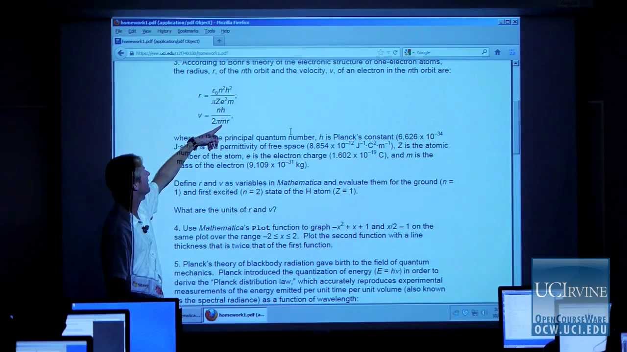
I thought I’d start out by asking if anyone has any questions or anything you want to discuss before we move on everybody got the homework then I hope not you haven’t even seen it yet okay so today we’re going to start out with an introduction to one of the most useful things that you’ll learn how to do using Mathematica and that is to make nice plots right so we all know a scientists that cleverly plotting data is a very nice way to convey a message and the message is best conveyed when you have a very meaningful and informative plot and so what I’m going to do today is introduce you to some a few features that will help you to begin to make nice-looking XY plots soap lots of functions of one variable and then a little later in the course will learn how to make 3d and even 4d plots and like I say I think this is one of the more valuable things that you’ll learn how to do all right so we’re going to start with a very simple example and what I’m going to do is show you how to plot a simple function so it’s going to be the sine function and we’re going to do it over one cycle so it’ll be from 0 to 2 pi alright and the name of the command is called plot this is the very simple plotting command for plotting a function either one that exists in Mathematica or one that you’ve defined and we’ll learn a little later today how to define our own functions and in its simplest form all you do is you say what’s the function you want to plot so in our case it’s going to be sine X and don’t forget that arguments to functions go in square brackets and then we need to give a range okay and by the way the variable doesn’t have to be X this is just a very common one to use it could be why it could be t it could be a it could be your name just so long as you’re consistent in referring to it alright so then I put a comma and then I put a range and this is going to be our first introduction to the use of the curly braces and as I think I previewed to you last time there are lots of different ways to use parenthesis braces and square brackets in Mathematica and braces are generally used to enclose lists and in this case we need to make a list of what’s the variable so we’ve said sine X so we should put X and then we put the minimum and maximum value over which we want X to be plotted so I’m going to go from 0 to 2 times pi remember pi is capital P lowercase I all right and then I close my square brackets and I enter and if you did it right congratulations because you have your first plot in Mathematica and so let me start by thing just a couple of things about it so first of all there is unless you specify otherwise a fixed dimension to the plot okay so there’s a mathematic it decides to use a certain amount of real estate in the vertical direction and then it by default uses about 1.6 times that in the X dimension so you get this rectangular plot and if you wish you’re certainly free to change this and many other attributes of the plot and I’ll show you a few and also show you how you can use documentation to unravel and uncover universe of possibilities for customizing your plot now the next thing is that notice that this sine wave fits very nicely within the plotting frame in general mathematica is going to try to fill as much of the plot as possible and so it’s going to adjust the limits in why so in this case from minus 1 to 1 that happens to be the limits of the function and X so as to use as much of the plotting frame as possible now this isn’t necessarily what you want and as we’ll see you can change that too okay and then the third thing that I’ll mention here is that mathematica has when you first fire it up a default coloring scheme that it uses and according to that default coloring scheme the first curve when you’re plotting plots in a given plot frame is going to come out blue once again this is something you can change and I’ll show you a couple of things ways that you can do that alright and then if you plot another curve which we’ll do in just a second it will come out in a different color okay so that’s kind of useful to know if you’re plotting multiple plots all right so this is very simple a plot and you can see that the command for it is is also very simple okay so what can we do now well this is a good time for me to emphasize something that you should start thinking about all the time which is as soon as you do anything significant as you’re working you should save your file all right so if you haven’t already seen how to do that let’s go ahead and do it now all right so what we’re going to do is uncover the menu here and then I’m going to say file save as and if i click on local disk there’s a folder called save here ok so in on these lab computers you’re allowed to save files in that directory alright so let’s go ahead and click on that and then you can put in a name alright so yesterday I saved a file called Doug 1nb today i’ll call it Doug 2nb you can call it whatever you want ok now another very important thing to keep in mind is that this file may not live very long after you leave the class okay in principle there they wipe these disks all these safe here directories automatically every 24 to 48 hours so the next thing you should do especially when you’re working on your homework and double especially when you’re working on your exams is to save a backup copy okay so all of you have probably been using computers for some time now and I would bet that most of you have some tales of woe about how you’ve worked for hours on some precious document right near the deadline and the computer crashed or the program crashed and you lost everything and you cried and you were really stressed out about it so what I recommend that you do to avoid that stress is to get into the very very good habit of making backups now in this course I can recommend say three that are very easy and take a very small amount of time one is just immediately email a copy to yourself another is create a Dropbox on your eee that you have waiting for you and upload a copy of your file to your sake m5 miscellaneous Dropbox and another thing you can do is you can have a thumb drive at the ready in the computer and move a copy over to your thumb drive every now and then to create a backup in this class losing your data because of a computer crash is kind of like turning in at paper late because your dog ate it it’s not an acceptable excuse okay so I’ve given you three good ways to back up your data and I will assume from now on that you’ll be doing so all right okay now back to our plot so the next thing we’re going to see how to do is how to plot two functions at the same time okay so the way you do that is you make a list of the functions that you wish to plot and so a list is enclosed in curly brackets so I’m going to put some curly brackets around this and then I’m going to add the second function which in this case is going to be cosine coasts of X and now if i press enter you see that i have two curves now how do you know which is which well first of all you should know the difference between cosine and sine but if you didn’t you could infer it because as I said Mathematica always draws the first one with the blue and now you can see that by default it draws the second one as purple okay alright so there’s a an introduction to plotting more than one function now I want to show you another way to plot something so this in it will be if you like an arbitrary function of your choosing and then we’ll see how we can manipulate some of the attributes of the plot because this plot is not extremely informative right it doesn’t have any axes labels it doesn’t have any units it doesn’t have a title it doesn’t have a legend and unless you knew that the blue curve was first in the purple curve was second you may not know which is which so we’ll have a quick look at a few of the various ways that you can customize your plot to make it much more informative now before I do that though I want to just introduce you to the Documentation Center in Mathematica this is an extremely useful resource you may not use it too much in this class because as i said i’m going to show you how to do everything that you need to know in this class but in future you may want to look up how to do things or even in this class you may want to look up how to do some snazzy things that i’m not going to teach you just because there’s not enough time okay so what you do is you go under the help menu and then if you want you can search for anything you want okay so suppose you were interested in finding out more about the plot command the various options that you may have just type in plot hit return and notice that the first thing to come up here is documentation on the plot command but you also can take a tutorial if you want this is often available and there are additional guides like a general algorithms for data visualization etc etc so let’s go ahead and click on this and you see that you get first of all a very very basic introduction to the syntax of the command and then there’s this box that says more information and usually the useful stuff is in that box and so now if you look at this list of things these are all lists of options that you have for changing the attributes of your plot and it looks in pretty intimidating but most of the time you won’t care about most of those things I’m going to show you a few of these but I just want to let you know that this exists because you may be curious and one away sometime making your plot look really super cool ok now another thing that’s occasionally fun to look at is the examples all right so these just generally show some very simple things it’s by no means exhaustive and then down at the bottom they usually have something called neat examples so this one’s particularly cool because it’s actually a chemistry example and this may not look familiar to you but as soon as you take chem 131a you’ll know exactly what this is this happens to be a very nice representation of the first one two three four five six seven eight wave functions or I guess those are the probability amplitudes for the harmonic oscillator which is a simple model for molecular vibrations has anybody heard of that before aha are you in chem 131a or took it already know okay cool all right well you’ll you will get a massive coverage and introduction to that in chem 131a those of you who are in that course will be getting this probably within a couple of weeks from now alright but anyway you can see that if you really wanted you could make such a beautiful plot yourself in Mathematica and it’s not that complicated okay so that’s the Documentation Center and I encourage you to consult it from time to time like I say for the most part though you won’t need it in this course alright so next thing we’re going to do is we’re going to plot a function that we define ourselves in the plot command itself and then will manipulate it okay so here what I’m going to do is I’m going to say plot and then instead of typing in a predefined function like sine or cosine I’m going to plot a an equation for a parabola so it’s going to be 2 times X minus 4 quantity squared and then plus 1 okay and I’m going to plot this between x equals 3 and x equals 5 okay now what should this look like well it’s a parabola that’s going to be displaced along the x axis by 4 and along the y axis by one all right so let’s go ahead and let it rip and there you have it and as before mathematica chooses the limits while we chose the limits of X but chooses the limits of Y so as to fill up as much of the frame as possible with the graph and you can see that it’s chosen to use the lower why limit as one alright so there’s your parabola now what if you wanted to represent this in a different way so suppose you’re teaching someone how to interpret the equation of a parabola you might want to plot it in such a way that you can easily see that it is in fact displaced by 4 and x and x 1 and y in other words you may want to plot it so that the origin of the plot which here was chosen for us it happens to be 3 and X and 1 in Y is at zero and zero so you can really see that it’s displaced from the origin well that’s something that’s easy to change and this will be our first introduction to a long list of potential plotting options okay and it’s also an introduction to a new piece of syntax so if you want to change the origin or specify the origin you use an option called axes so its capital a and then origin with a capital o and then what you do is you use a narrow construction to point to where you want the origin to be and the way you make an arrow is you make a hyphen and then a greater than and then you put the coordinates that you want the origin to be at all right so I’m going to do 00 and I put those in curly braces all right and now if I enter that notice that it’s drawn the same curve but now the origin of the plot is where I told it 00 and now we can see very clearly by looking at the plot that it’s displaced the minimum is displaced by 4 and x + 1 and y ok so it’s exactly the same data but it’s plotted in such a way as to convey a new point all right it’s a very simple example of a manipulation that you may want to do from time to time to make your plot convey the message that you wish to convey okay now one more comment we’re going to be learning more and more of these options and you might be thinking man this is super confusing i don’t remember when to use curly braces when to use arrows what the words are that I’m supposed to be using to do this or the that don’t worry about that because the best way to make complicated constructions in Mathematica is to look at an example and then modify that example to do what you want to do and as I already emphasized last time anytime you’re doing anything in this class you will always have available to you the notes from the class and everything that I’m going to ask you to do there will be an example of that in the notes okay so don’t get bogged down memorizing all this impacts all right so another thing that you can do so here we’ve changed the origin okay another thing that we may want to do is we might want to actually manipulate the range over which the function is plotted okay so here mathematica chose to plot it between 0 and 3 and since we didn’t specify the range of X it uses the full range that we specify which was 325 plus if there’s an origin it also includes whatever’s between that and the origin okay so to customize the plot range what you can do so let’s go ahead and mouse this in here so ctrl-c to copy and then ctrl-v to paste so there’s another option which is called plot range so plot and then capital R a n GE and hear what we need to do is include two ranges 14 x and 1 for y so suppose in X I want to go between one and ten alright so that’s the X range now I have to include another set of curly brackets and then put a comma and specify the range of Y so Y I may wish to make let’s say just for fun Oh point 5 25 okay so if we enter whoops i need another curly bracket here then I get this plot okay so there’s no particularly compelling reason why I chose that range other than just to show you that you can change it and as you see the plot goes between 1 and 10 and 0 point five and five as we told it okay alright what else can we do well I’m going to start by going back to our very simple plot I’m just going to nuke all this stuff here and re-enter all right so so far all the pots we’ve made our pretty lame actually because we don’t know what we’re plotting all right so how can we specify what we’re plotting well one thing we can do is we can label the axes okay another thing we can do is we can actually give the plot a name or a title a label okay so now I’ll show you how to do that so these are additional options and the first one to label the axes is called axis label and then we need an arrow and then we need to make a list of two names one for the each axis and these should be in quotes because they’re going to be written exactly as whatever you put in the quotes so in the first set of quotes for the x axis I’m going to call it X and for the second axis Y I’ll call it Y now if you enter that you see that you have a microscopic label over here for X and another microscopic label here for why and I’ll show you in a moment how you can change the sizes and fonts and things like that okay now what about the label well we can put in another option it’s called ironically enough plot label arrow and then in quotes you put in whatever you want so you can say this is a cool plot or whatever you want to say about it you might want to say this is not a cool plot okay and if you enter that now you see that you have axes labels and a plot label now as you can see I wear reading glasses so for me these microscopic axes labels are very hard to see without putting my glasses on so if I want to be able to read my plot without my glasses I need to make those bigger so i’ll show you how to do that in addition i don’t know about you but i’m not a big fan of the times font which is the default font that you get when you make plots i actually like the Sun Surrey faults like helvetica you want to change that no problem here’s how to do it alright so more options which we just tack on to the end now the syntax for changing these things looks pretty intimidating but like I say don’t worry about it you can look at the notes for examples so these attributes things like the font face the font size these are what’s part of a broad array of attributes called base style okay so the way we change them is we say face style arrow and then we have some curly brackets because we’re going to make a list of things that we want to modify all right so the first is what’s called font family and I’m going to put it website spelled it wrong font family and then I put it in the arrow and then i’m going to change it to one of my favorites Helvetica okay and then the other option i’m going to put in is the font size arrow and I’m going to crank it up to 16 16 points I think the default is 10 all right and i got an error I forgot the curly bracket before the 16 we’re here I don’t need a curly bracket there I have a curly bracket here that includes both of the base style options and well we could see what it has to say here so you know this is going to happen a lot right and it’s good for you to see how to fix things so you know how to fix it oh yeah I don’t need quotation on the numbers that’s right thank you alright let’s see if that works ok there you have it alright so now you can see we have the Helvetica font and you can read it the axes labels are bigger too okay so as time goes on you know you’re going to learn how to make more and more modifications to your plots in the homework I’ll often give you very specific instructions about what I want you to do and so you should always do that but in addition i encourage you to let your creative juices flow and use colors or plotting attributes to spiffy up your plots to your heart’s content you’ll impress your TAS when they’re grading so the minimum requirement is include all the elements that I tell you to but after that the sky’s the limit as long as you don’t you know modify the information content of the plot okay all right now let’s do some other things that are very important if we want to make scientifically meaningful plots ok so now I’m going to go back to our previous example of the sine and cosine all right so I’m going to Mouse this in and put it back control be okay and we’ll go ahead and answer that to remind ourselves what that looks like so here we have our two curves alright and what I want to do is I want to play around with the curves so in various ways so as to make them distinguishable more distinguishable okay and also while I’m at it I’ll show you how to make plots in black and white or grayscale this is sometimes nice because if you have say a black and white printer if you were to plot these two curves they probably be really hard to tell apart so you may want to make your curves in black and white and then use other attributes like line thickness or dots and dashes and things like that to make the plots look different okay so we’ll do that first alright so now what we’re going to do is we’re going to make both of these curves black alright and this can be accomplished by using an option called plot style ok and I’m going to put some current whoops it has to have an arrow and then some curly brackets and then for each of my plots I’m going to specify some attributes inside plot style ok so one of those can turn these plots into what are called gray scale alright so let’s let’s do that so for the first plot i’m going to say gray level and i’ll explain to you how this works in just a second bracket 0 so that’s an option for the first plot and then if i put a comma then i can specify an option for the second plot and i’m going to make it the same and if i enter that you see that I converted both of these plots to black so gray level is a number between 0 and 10 is black one is white ok so if i wanted to make one of these plots gray so as to make a distinguishable from the other one so for example the second one I could change this number to save point five if I do that then you see that the cosine curve actually comes out grey but still that’s not a very impressive difference so what I’m going to do instead is I’m going to go ahead and keep this one black except now i’m going to add an additional option for the second curve that will turn it into a dashed line ok so if i’m going to added an additional option i have to put in another set of curly brackets so that i can make a list of options for the second plot within those ok and to make a dashed line all i have to do is say dashed okay and if i enter that I see that it didn’t do it and one problem is i have this curly bracket in the wrong place ok so there you have it alright so that’s kind of nice and you know i’m not going to go into all the things that you can change but if you look in the documentation you’re there are many other options besides dashed and you can also change the size of the dashes for each curve you may want to make several curves with different sized ashes so as to distinguish them okay so we have a question I’m sorry I can’t hear you well to change back to blue and red you just remove all the stuff that we did to change it away from blue and red okay so here I’ll show you how so we mouse this back in and if we could just go down here and remove all this stuff that we changed we’ll go back to the default okay all right so it may not be obvious to you why you might want to do this I guess the this most straightforward example is you may have a black and white printer and you want to make a meaningful plot another is this maybe isn’t so relevant to you at this stage of your life but when you publish stuff in journals sometimes the publishers will charge you a lot of money to get your figures plotted in color and so whenever you can make plots in black and white you tend to do so to save money and because we have things like dashes and as I’ll show you in a minute line thicknesses things that we can change we can still make perfectly beautiful meaningful plots without using color at all nowadays color printers and color toners are pretty cheap but when i first started my education color was very hard to come by and when you could come by it it was very expensive okay all right what else can we do here well we can change the thickness of the lines all right so all what I’ll do is I’ll change the thickness of the first curve so I’m going to put in curly brackets around the sky and then there’s a command or an option called thickness and there’s a number that goes inside and this number happens to be the fraction of the plot with okay so if i put in 0 point 0 1 what that’s going to do is it’s going to draw the first curve in solid and the thickness of the line will be one percent of the width of the plot okay so if you enter that you see that you get a fat black curve for the sign okay so these are just a couple or few of the various ways that you can manipulate your plots to make them contain more information now the next thing I’m going to show you is well actually i’ll show you a couple things the next thing i’ll show you is how you can make the plot frame look a little bit different this sometimes is preferable from people like to have a frame that goes completely around the plot okay now the way you do that is you put in another option the default is to not put one right here we’ve got just the two axes if I put in an option here that says frame arrow true it’ll draw a plot frame ok notice the difference you may want to do it you may not if you do this is how you do it now one little idiosyncrasy about having the plot frame is that the way you label the axes is different I didn’t invent this so don’t blame me but i’ll show you how to label the axes so remember when we had the regular plot that doesn’t have the frame we label the axes by saying axes label here if we have a plot frame that doesn’t do anything what we have to do is say frame label ok so let’s try that so we say arrow and then after that it’s just like before we put in the labels we want so I’ll just say x and y alright if you do that notice it puts the labels at the middle of the axes which is aesthetically pleasing to some and suppose you want to label the plot it’s the same command as before it’s called plot label so maybe you want to say my favorite trig functions okay all right now the next thing is again so far we’ve done a very nice job of distinguishing our two plots but if we hadn’t taken trigonometry class yet we wouldn’t know which one of those is which so what we want to do now is we want to include some labels that tell us which curve is which okay and one convenient way of doing that is by using what’s called a plot legend ok so what a plot legend is is it basically a little sample of each curve and next to each sample you have some name that you give it that tells you something about what you’re actually seeing here so for example I might want to label this one sine of X and this one cosine of X all right now plot legends for some reason the geniuses at Wolfram research decided is not something that you’re going to want to do all the time and the way Mathematica is is written it’s it’s actually a very very big and complex program and if you try to load all of its capabilities at once into memory you’d be using up a lot more memory than you really need to to do most things well to do pretty much anything you want to do so what they’ve decided to do is to load in when you fire up the program you load in a small number of what are called packages that are you’re likely to use a lot and then there’s additional capabilities that you use less frequently that are available but they have to be loaded okay and it happens turns out that plot legends are one of those things so if we want to include legends in our plot we actually have to load what’s called the plot legends package okay so the first thing I want to do is just to show you how it is that you can see what’s already loaded so if you type dollar and then packages and enter that you get a list all right and this list probably doesn’t mean a whole lot to you and it certainly doesn’t mean a whole lot to me these just happen to be the names of the packages that are loaded by default when you fire up mathematica okay so one of this this one looks kind of familiar that’s the searching program all right now if we want to load a package it’s got a funny syntax but again you always have examples to look at we do the following we say less than less than and then we say the name of the package so in this case it’s going to be plot legends capital L and then you put a backward single quote which is the upper left hand corner of your keyboard all right and now you enter that now if you type dollar packages again what’s the with a capital P and no a then you see you have an additional one that you didn’t have before which is called plot legends and now you can actually use commands that are required in order to install a plot legend so let’s go ahead and mouse this guy in here and put it down here and enter it okay and now what we’re going to do is we’re going to label these two curves with a plot legend okay now the way you do that is you add an option and by the way this option will not be available to you until you load the plot legends package where you say plot legends plot legend arrow and then you have a list in our case it’s going to be two items because we have two curves a list of the names that you want to give to each curve okay so for the first one I’m going to call it sine of X and that should be in double quotes sorry and the second one will be cosine of X and ah my quote here I don’t have a closing quote here okay there it is all right by now you’ve probably already noticed that if there’s anything wrong with your command to like missing brackets and things that you get these color-coded alarm bells going off so they kind of help you to figure out what you’re missing all right so let’s try that there you go so here is a plot legend that tells us that the blue curve is signed and the purple curve is cosine this is very very useful right for making a meaningful plot now it’s not so nice is that by default this thing is placed so that its center is at the lower left-hand side of your plotting frame which is in many cases not a very pleasing place to put it so we’ll see how to move it in just a second another thing that I don’t like about this default legend is that they have this shadow which later on we’ll learn how to nuke that and also you can will learn how to change spacing between these guys and you can get rid of this frame if you want so there’s lots of things you can do but for right now I just want you to see how to put it there and then move it someplace so that it’s out of the way all right so now if we want to move it what we do is we put in another option which is called legend position except we have to spell it right arrow and then we put in coordinates so we have to put in X and the y in and what these coordinates are is they’re coordinates in fractions of the plotting frame all right so if I want to move this guy all the way off to the right so that’s not sitting on top of my plot I should put a number greater than 1 and then I can play around with the vertical to get it to a place where I like how it looks so let’s try 1.1 and then I’ll put in minus 0.3 so that’s going to be the Y where it is in the Y and if you enter that you see that now your legend is in a much nicer place where it’s not sitting on top of your plot okay no because these coordinates are in units of the dimension of the plot so what 1.1 means is it’s point 1 beyond the edge of this in terms of the width of the plot okay yeah but usually when you do when you’re dinking around with these things you kind of play with the numbers until you get something that you like so I just so happen to like this because this is roughly centered on Y and it happens to be off the edge of the plot change the numbers see what happens by the way that’s something I should encourage you all to do while we’re sitting here dinking around you don’t have to do exactly what I do if you’re curious to see how something works play around with the things the worst thing that can happen is that won’t work okay all right any other questions okay so this is all i’m going to say for now about plotting okay this will be enough to do a good job on your homework and as time goes on we’ll see new new ways of making plots and we’ll get more and more sophisticated but already right now you can make really cool plots and hopefully you’re all very happy with yourselves okay now we have a couple of other things that we need to do in order to be able to do the homework and these are things that we’re going to use a lot so if you have any questions whatsoever next ten minutes or so please make sure we can’t get them answered okay so the next thing we’re going to do is we’re going to learn how to assign variables okay so let’s let’s see you have to do that so the assignment of a variable works the following way name of your choice equals something of your choice that you wish to associate with that name and it’s kind of like algebra right and then once you’ve assigned a variable you can use it subsequently and you can change the value if you want and use it again okay so your introduction is the following what I’m going to do is I’m going to define a equals 2 and B equals three and then I’m going to add a plus B i’m going to multiply a times B and I’m going to raise a to the B power just so you see how this works okay so if we enter this we get a sequence of numbers this one is just telling us that we’ve assigned a 22 this one tells us we assign b 23 this one here is the result of a plus B this one’s the result of a times B and this one’s the result of eight power be okay now I want to show you one more thing because you know here we’ve executed a bunch of commands in a row and we have to be you know sort of like map them onto each other it’s kind of a pain right so there’s a very useful thing to be able to do because you don’t necessarily want to see the results of all these things right you might want to hide the first two for example the way you do that is use a semicolon this will suppress the output of a given operation so to see how that works let’s go back and put a semicolon here and a semicolon here Wow and do it again now you see that the initial assignment of a and B has been hidden and in general there will be lots of things we don’t want to see we may want to do a whole bunch of calculations and only see the last result all right and then we get the things in a row here okay all right now what else could you another thing we can do is we can make expressions all right so now I can say for example x equals 2 times a plus B alright and if I enter that I get seven because I’ve assigned to 2a so two times two is four and have signed B equals three so 4 plus 3 is equal to seven all right now suppose I want to go back and just have X defined as an algebraic expression but without any numbers assigned there’s a very useful command that allows you to remove the assignment of a variable name to a number and this is very useful if say within the same notebook you’re using the same name for a number that may you may use it in one set of units in one place and another set of units in another place so the numerical value changes so for example the gas constant might be you can have that in SI units or you can have it liters atmospheres moles Kelvin and as you know by now in chemistry and physics and sciences we oftentimes use the same letters to refer to different things okay and if you’re using the same letter in multiple places in a notebook you may forget that you assigned it to one thing somewhere and you’ll get some bogus answer down below when you try to use it in a different context so there’s a very useful command that I will use a lot when we start doing more complicated things which removes the assignment of a variable and that’s called the clear command alright and so the way I can do that as i can say clear and suppose I want to clear the a ok put a semicolon and now I ask what is X hey that wasn’t supposed to happen Oh xrx was already assigned let’s let’s clear a and X and now you see X is no longer defined if I look at a it’s no longer defined if I say x equals 2 times a plus B notice i get 2a plus 3 because b is still assigned to three okay if i clear be and then asked what sex I get back to my right oh I’m sorry so actually this is showing something that’s really it’s gotten me confused today and probably get me confused and you confuse later x was already defined as 3 plus 2 a here right yeah so I have to clear it again and redefine it if I want to use it all right so if I clear X and now I say x equals 2 times a plus B now I get back to my pure expression so you have to be really careful when you assign things if you’re going to make assumptions about using those expressions later it’s always helpful to to clear things and reassign your variables if necessary okay alright so those are some simple examples of defining variables assigning numbers to them and then using them in expressions okay and you’ll get to do some of that in your homework all right now the next thing and this is another very very important thing that will be doing a lot and so I suggest you pay close attention is we’re going to learn how to define functions alright this is extremely useful and so the first thing we’ll do is we’ll take that parabola that we plotted earlier and we’ll assign it to a function which i’m going to call f of X and what I want you to do here is pay very close attention to the syntax the way the definition works because this is probably one of the most common sources of mistakes that will encounter this quarter all right so what I’m going to do is I’m going to define f of X equals that parabola we saw earlier all right so the way I do that is I say give my name it doesn’t have to be f it could be whatever you want f and then remember arguments of functions come in square brackets now next thing I do is I put in the argument and here’s one thing that maybe it doesn’t make sense but you have to do it otherwise your function won’t work when you define a variable argument to a function you have to put an underscore why is that well why is that is because you may have several arguments to a function but some of them you may wish to remain constant or you may want to put in a particular value so that it’s not actually an independent variable this is so you can distinguish between true independent variables and some parameter or something alright so if you want to indicate the variable when you define the function you have to put in the underscore and leaving that out is a great source of error the next thing is when you’re first defining the function you don’t just use the equal sign the function definition is special and it has colon equal ok all right now we define our function so at this point we could put anything we want in here but I’m going to put in that parabola 2 times X minus 4 quantity squared plus 1 okay so I enter that and if I did everything right usually I won’t get any feedback now i can check at any time to see if I’ve assigned f to a function there’s a if i say ? f it will tell me whether or not its sign and if it is assigned it will tell me what its assigned to so if i enter that you see that I’ve this just means it’s a globally defined function and it tells me how I’ve assigned it and so I can actually check to make sure it looks like what I want it to look like okay now once I’ve defined this function I can do lots of things with it so for example suppose I want to evaluate it for a given value of x like say x equals 1 all i have to do is to give me f of 1 and you see i get 19 does that make sense x minus 4 is minus 3 squared is 9 times 2 is 18 plus 1 is 19 okay you can put in whatever you want suppose you say f of pie if you put in pi as I told you last time Mathematica will keep the exact result so in this case it just puts in the pie if I want a numerical value for that I can say in bracket percent like we learned last time and so there’s my numerical value another thing i can do is i can plot it by referring to X I mean F so I can make the same plot as we made before by saying plot f of X comma and then X goes from three to five if i do that i get the familiar plot that we made before okay so this is a very very useful thing to be able to do now yes okay yeah you just say clear put in brackets and list them off any other questions yeah you sure okay alright so the next thing I want to do is I want to define a quite complicated function that’s relevant to chemistry and the reason I want to do this is because i want to emphasize to you that oftentimes the way we type functions in in this command line of Mathematica looks a lot different from the way it’s written in the textbook or on the homework assignment or whatever now a little later we’ll learn how to type set our things but for now anyway I want to teach you the brute force way to do it and the main point of this is that as time goes on we’ll be working with fairly complicated functions and there’s lots and lots of ways that you can make mistakes and I so I want to point out a couple of those here alright so what we’re going to do I’m going to write the function on the board is we’re going to plot something that you’ve seen before you may not have ever seen the formula but you’ve certainly seen the function and it’s called the maxwell-boltzmann distribution does that ring a bell to anyone okay well I’ll remind you since I know you know what it is this is the probability that comes from kinetic theory that an ideal gas molecule has a certain speed and you may remember seeing this in your text G chem textbook so it looks something like this all right it’s a distorted bell curve okay and often the variable use for the speed is you and that’s in meters per second in SI units and then the y axis is often called F of U or P of U and it’s just the probability that a gas molecule and an ideal gas has a speed within a small increment around you okay now the formula is as follows and this is what we’re going to type in and then we’re going to plot it and hopefully you’ll see that it’s kind of cool because you can quickly remind yourself of some things that you were probably asked about on your G chem final exam in chem 1a probably all right so this formula looks like this okay so if you look up the maxwell-boltzmann distribution in your favorite textbook that may have it oh yeah let’s turn on the light oh thank you did I turn off the light oh okay there we go alright so for pi times quantity M over 2 pi r T M here if we’re in SI units would be the molar mass in kilograms per mole r is the gas constant 8.314 joules per kelvin per mole t is the absolute temperature use the speed in meters per second and that’s everything ok now another thing about somewhat complicated formulas is that it’s never a bad idea to see if you can’t predict before you actually plot it what it might look like that’s not always going to be the case but whenever you can it’ll be helpful because there’s a lot of ways to screw this up when you enter it in and when you make a plot you want to be able to kind of tell whether or not your plot is bogus or it seems to be correct so let’s ask ourselves what does this thing look like at various when you is very small well when you is very small how does this thing look this exponential it goes to one so the dominant functional behavior is u squared u squared the parabola so it should look like a parabola it’s small you what about it large you at large you this guy starts decaying very quickly because it’s got u squared in an exponent so the large you dependence of this function is going to look like a decaying a fast decaying exponential so that’s why you have this tail here ok so that helps so that when we make a mistake typing this in will recognize it and when we get it right we’ll say mm-hmm all right so let’s go ahead and type that sucker in and then we’ll play around with it a little bit all right so notice I already defined F here and I want to use the same variable so to keep from getting in trouble i’m just going to write a head right away say a clear path all right okay now i start typing so f of you remember underscore for the variable colon equals then i have four times pi capital pie and then times parenthesis another thing that i want to recommend to you is even though the formula over there has some capital letters and usually you can get away with using capital letters all of Mathematica is predefined stuff variables and functions they start with capital letters and so to avoid accidentally stepping on one of those are using them where you don’t want to and getting an error I recommend that you always begin your variable and function names with a lowercase letter even if it doesn’t look pretty ok so I’m going to go ahead and use little m for the mass so m and then divided by 2 pie R T so I say 2 times pi times little R times little T ok yes so already one of you see is a problem with this so how is this going to be interpreted what it’s going to do is it’s going to divide n by 2 and it’s going to multiply all of that by PI R T which is not what that formula says that formula says multiply all these together and then divide em by that so in order to make sure that that actually happens I have to use parentheses to keep the pieces of the denominator all together okay all right now I want to raise the whole thing to the three halves power so carrot and then to make sure i get my three halves i put that in parenthesis and now i want to multiply by u squared and then finally i have to put in that exponential so remember capital e and then carrot and some parentheses and now i’m going to use parentheses to group the numerator and denominator of the argument to the exponent together so the first one is minus M times you carrot two parentheses and then divided by parenthesis two times R times T alright so does that look right let’s enter it okay now what we’re going to do is we’re going to plug some numbers in and we’re going to see if it looks like what we remember from G chem alright so I’m going to do n 2 so it’ll be like a typical gas molecule in the air in this room alright so i’m going to say the mass is equal to zero point zero two eight that’s the molar mass of n2 in kilograms per mole okay i’m going to put a semicolon because i don’t want to see it i’m going to put in room temperature so 300 kelvin all right and what else do i need to specify are the gas constant so i’m working in SI units so i’m gonna say R equals 8.314 and that’s joules per mole Kelvin all right and now what I’m going to do is I’m going to plot f of you and what you may or may not remember from G chem is that the average speed of typical low-mass gas molecule at room temperature is a few hundred meters per second so that tells me that if I want to see the full range of this curve I might want to go out to say a couple thousand that’s going to be my range for you so you goes from zero to two thousand alright and let’s let it rip and see what happens and sure enough I get something that looks like the maxwell-boltzmann distribution look familiar by the way another thing that you can do any time in this class is if you need to go look something up somewhere to check your result because it you maybe you think I’ve seen that before but I don’t remember what it looks like feel free to Google Wikipedia whatever you want in this class I encourage that ok so anyway if you were to Wikipedia the maxwell-boltzmann distribution you find a curve that looks like that all right now now we have a learning tool because now we can say oh I forgot how that changes when I change the mass so suppose I want to say hmm what happens if i look at a heavier gas molecule like chlorine cl2 well i can change the mass so let me go ahead and just well let’s go down here so we can see it so now i’m going to change the mass to M equals zero point zero seven nine that’s the molar mass of chlorine cl2 in kilojoules or kilograms per mole and now I can just mouse this guy back in and put it here andrey plot and now i could remember what happens when I change the mass of a gas molecule notice that I’ve moved the most probable speed from over around 500 down here to you know around 300 and this makes sense right because we remember from G chem that heavier molecules move slower at a given temperature than lighter molecules what if you wanted to see the effect of temperature what’s happens as you crank up the temperature to the speed of a gas molecule it increases alright well let’s go down now and have a look at what happens if we change the temperature to a thousand Kelvin and then reap lot so now this is going to be chlorine at a thousand Kelvin and sure enough you see that the peak moves to the right and the distribution becomes broader so you can compare these two to see the temperature effect all right so there you have it that’s a somewhat complicated looking thing there and we successfully typed it in and we actually used it to dust the cobwebs off of our knowledge about kinetic theory of gases all right okay so we have a few minutes left and what I’m going to do now is just show you a couple more little miscellaneous things that you may find useful in your homework and then I’ll spend about three minutes going over telling exact telling you exactly how to do your homework okay so first of all everything we’ve done so far is we’ve just put in a bunch of random commands in our notebook now what you’d really like to be able to do if you say are doing your homework and you want your TA to understand which problem you’re working on and maybe even want to provide some information about what you’re actually doing so that if you do happen to make a mistake they can at least tell whether or not you knew what you were doing or supposed to do you want to add information in your notebook that’s not actually executed but is just meant to be informative this is useful if you have a very complicated notebook and you want to give it to somebody else and have them be able to read through it and understand it okay so there’s a couple there’s lots of ways to do this i’m just going to show you too okay so the first is and simplest is to use what’s called a comment okay so a comment you can type directly in without doing anything else and the way that works is if you say parenthesis star that’s a signal to Mathematica to ignore everything that comes after it so for example here is a plot mb distribution for cl2 at one thousand Kelvin now to end the comment what I do is I say star parenthesis all right and now if I enter that nothing happens because it’s ignored but it does appear in the notebook all right so you might want to say you know you might want to put another line in here that says this is homework one problem one oops and that will help your ta to see what it is you’re actually working on ok so that’s one way another way which I find that most students prefer because it’s a lot snazzier is you can go anywhere in your notebook and you can introduce a different type of area ok so so far all we’ve done is we’ve been in this sort of command mode but you can change in two different modes so for example format style I can change from input mode to text mode okay and now I could say this is a text box and if i want i can do all the usual things here like change the font and the font size I can change the color of this to make it look different so that my text is say with a lime green background as opposed to just the white you can play around with this stuff and make your notebooks look really snazzy and easy to read okay so you’re welcome to do this you don’t have to but I do advise at least at bare minimum the use of comments to make your notebooks as easy as possible to read all right now let’s have a look at the homework alright so there should be a drop box set up for you this is section a so it’s going to say homework 1a and when you’re done with your homework you can turn it in there by the deadline is saturday 5pm you should be able to get it done tomorrow easily within your to our lab session so here it is it’s five problems the first two problems are just to give you practice on putting parentheses in the right places so first one you’re going to see the difference between 2 to the 3 quantity to the 4th and 2 to the power quantity 3 to the 4th you should get quite different numbers as you may be able to anticipate and then you can do this fraction of fractions with exponents okay and for the second one you’ll get an exact representation which is going to be a ratio of a couple of integers and I want you to convert that to numerical value with 15 places using the N command alright then the next thing I want you to do is define these two things ok so these happen to be the radius and velocity within the Bohr model of the atom for the enth bore orbit where n is the principle quantum number M is the mass of the electron RS is this here Z is the nuclear charge which for atomic number which for hydrogen is one this year is not the base of the natural logarithm so here’s an example where we use the same symbol for two different things as I say here e is the electron charge in coulombs so all this is in SI units h is planck’s constant pi is pi and easy row which you can type in as if you want you can have little e0 next to it to make it different from E that’s what’s called the permittivity of free space and its numerical value is given here in SI units I’m sorry you can use whatever you want yeah as long as the formulas right okay now what I want you to do is to define these two things and then define the values of all the constants and then there’s going to be one left over that’s not defined that’s n the principle quantum number and then I want you to evaluate both of these for n equal 1 and n equal to so the ground state and the first excited state of the hydrogen atom all right so you can think a little bit about how best to plan that because you need our to calculate V you should define our before v okay and then I asked you and you can give your answer in a comment or a text box what are the units in my hint to you is everything’s in SI units so are as a distance in SI units and v as a speed in SI units you don’t actually calculate anything there you just think about what are the units okay next thing is I want you to plot this and this on the same plot I tell you the range of X and the only stipulation here is that the second one x over 2 minus 1 should be using a line that’s twice as thick as the first one all right so you can make whatever color you want I just want to see you change the thickness so you might want it to find a certain thickness for the first one and then twice that for the second one okay and then the last problem I’m sorry I’m eating up a minute or two of your time here is it looks complicated but it’s mostly because I’m trying to explain to you what it is that you’re going to be doing in case you’re interested but what this problem boils down to is that I want you to define this function and later I’ll teach you how to actually put things like lambdas in there so they look nice but for now you might want to just type it out lambda as a variable name so you’re going to define this function H plunks constant sees the speed of light those are given there k is boltzmann’s constant is given here so define that and and the constants and then you’re going to define another function down here which is also a function of lambda and I want you to plot those two on the same plot here’s the range of lambda I want you to use and I tell you the range of in the y-axis that I want you to use so that you can see the difference between the curves and put in a temperature of 5800 so what this is is that this formula here is the formula plunk derived for the radiant spectral radiance of a black body as a function of wavelength and when you were first learning quantum mechanics in general chemistry you learn that plunk introduced the quantization of energy equals H nu and he did that so that he could derive this formula which correctly describes the shape of the spectral radiance versus temperature and what you’re going to see is that it’s going to look something like the Boltzmann distribution is going to be a distorted bell curve now the reason that was so important is because it showed that his hypothesis e equals H nu was actually consistent with experimental data on black body radiation and this curve is the best that physicists could do before plunk came along this was based on classical electromagnetic theory and what you’re going to see by plotting these on the same plot is that this thing is really really wrong if this was correct there would be no such thing as darkness okay so in any case for us though it’s just an exercise in plotting two curves on the same plot and I forgot to tell you somewhere in the instructions it says you have to include a legend okay all right so good luck and joy and we’ll see you I guess on Thursday you